Why Karnaugh Maps Work
In section 1.2 we simplified Boolean expressions by hand and saw the problem with doing so: it depends on noticing things, and nothing tells you when you have found the smallest form. In this section we use a method that turns the search into a drawing exercise. It comes from a two-page paper that Maurice Karnaugh published at Bell Labs in 1953, and it is still taught in every introductory digital design course because it works. This first article explains why it works. The following ones use it.
The problem with algebra
Take a function with four variables and a dozen minterms. You can spend an hour applying theorems, arrive at something compact, and still not know whether it is minimal. A colleague starting from the same truth table might apply the rules in a different order and finish with a different expression, equally compact, or smaller. There is no clear stopping point.
Three things make algebraic minimisation hard: it needs insight into which theorem to apply next, it does not scale beyond four or five variables, and it gives no guarantee that the result is minimal. Karnaugh’s map addresses all three by turning minimisation into pattern recognition on a grid.
Adjacency is combinability
Start from something you already know. Two product terms can be combined when they are identical except for one variable that appears plain in one and complemented in the other:
$$A’B + AB = B(A’ + A) = B$$
Karnaugh’s question was: can the minterms be arranged on a grid so that any two minterms that can be combined in this way are next to each other? The answer is yes, and the arrangement is the Karnaugh map.
Gray code
A 4-variable function has 16 minterms. The obvious way to lay them out is a 4×4 grid with rows labelled AB = 00, 01, 10, 11 and columns labelled CD the same way. That does not work. Rows 01 and 10 differ in both bits, so cells in those two rows are not combinable, even though they touch.
The fix is to order the labels in Gray code, so that each label differs from the next in exactly one bit:
$$00 \to 01 \to 11 \to 10$$
From 00 to 01 only the second bit changes, from 01 to 11 only the first, from 11 to 10 only the second. With both axes in this order, any two cells that share an edge differ in exactly one variable, which is exactly the condition for combining them.
The map wraps around
Notice also that the last label, 10, differs from the first, 00, in only one bit. So the leftmost and rightmost columns are adjacent too, and so are the top and bottom rows. If you glued the left edge of the map to the right edge you would have a cylinder; glue the top to the bottom as well and you have a torus. Every cell on it has exactly four neighbours, and every pair of neighbours is combinable. Figure 1 shows the 4-variable layout with the minterm numbers and the two wrap-around adjacencies marked.
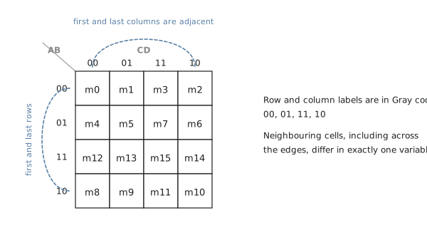
This wrap-around is what makes groups across an edge, and groups of the four corners, valid. They look scattered on paper, but on the torus they are a rectangle.
A two-variable example
The simplest case: a 2-variable function has four minterms in a 2×2 grid. Take $F = \sum m(1, 3)$, which is 1 when $A = 0, B = 1$ and when $A = 1, B = 1$. Figure 2 shows the map with the two 1s and the group around them.
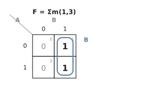
The two cells are in the same column, so they are adjacent and form a group of two. In both cells $B = 1$, while $A$ takes both values. $A$ drops out, and the group is the single term $B$. So $F = B$.
Check it algebraically: $A’B + AB = B(A’ + A) = B$. The map did in one glance what the algebra took two lines to do, and the saving grows quickly with larger functions.
What a group means
Every valid group of $2^k$ cells in a map is one product term. The term contains the variables that are constant across the group and leaves out the ones that vary.
| Group size | Variables eliminated | Literals in the term (n variables) |
|---|---|---|
| 1 | 0 | $n$ |
| 2 | 1 | $n - 1$ |
| 4 | 2 | $n - 2$ |
| 8 | 3 | $n - 3$ |
| $2^n$ | $n$ | none, the function is 1 |
The aim is always to cover every 1 with the largest groups you can. Larger groups mean fewer literals per term, and fewer terms mean fewer gates.
Why it scales better
For a 4-variable function with eight minterms in two overlapping groups of four, an algebraic simplification might take ten or fifteen steps. On the map you draw two rectangles and read off two 2-literal terms. More importantly, the method is a procedure rather than an art:
- Plot the 1s of the function on the map.
- Find the largest valid groups.
- Cover every 1 with as few groups as possible.
- Read a term from each group.
- OR the terms together.
Working engineers used this as their main minimisation tool from the 1950s to the 1980s, and it is still what you reach for when a small function needs simplifying on the back of an envelope. For large functions the same idea runs inside synthesis tools, as an algorithm rather than a picture, and the last article of this section looks at that.
Practice Exercise
Draw the 2-variable map for $F = \sum m(0, 1, 2)$, find the groups, and write the minimal SOP expression.
Solution
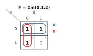
The top row, cells 0 and 1, has $A = 0$ constant and gives $A’$. The left column, cells 0 and 2, has $B = 0$ constant and gives $B’$. Cell 0 is in both groups, which is allowed and is what lets both groups be as large as possible. $F = A’ + B’$.
Check: cell 0 has $A’ = 1$, cell 1 has $A’ = 1$, cell 2 has $B’ = 1$, and cell 3 has both terms 0.
In the next article we work through two- and three-variable maps properly, with the full set of grouping rules and the vocabulary of prime implicants.