Module 5: Behavioral Verilog for Synthesis
Module 4 described circuits by wiring gates and by writing equations. Both make you think in gates. This module is about the third style, where you say what the hardware does at each clock edge and the synthesiser works out the gates. It is behavioural RTL, and it is what nearly all production Verilog looks like.
Still not a program
Every module so far has said that Verilog is not a programming language. This is the module where that is easiest to forget and most expensive to get wrong, because behavioural Verilog has if, case, for and variables that are assigned and read back, and it looks like C.
Two always blocks side by side are not two functions that run one after the other. They are two circuits, both powered, both running. If block A writes a signal that block B reads and block B writes one that A reads, that is a feedback loop in hardware, not mutual recursion. Keep the picture from Module 4: every always block, every assign, every instance is a machine bolted to the floor and running, and nothing waits for anything else.
The two rules
Everything in this module follows from two rules, and it is worth having them before writing an always block.
In a block clocked by an edge, always @(posedge clk), every assignment uses <=.
In a combinational block, always @(*), every assignment uses =.
They were not chosen for taste. They come from the way the simulator schedules events, and section 5.1 derives them from that, because following rules you do not understand gets you correct simple code and mysterious complex bugs.
The sections
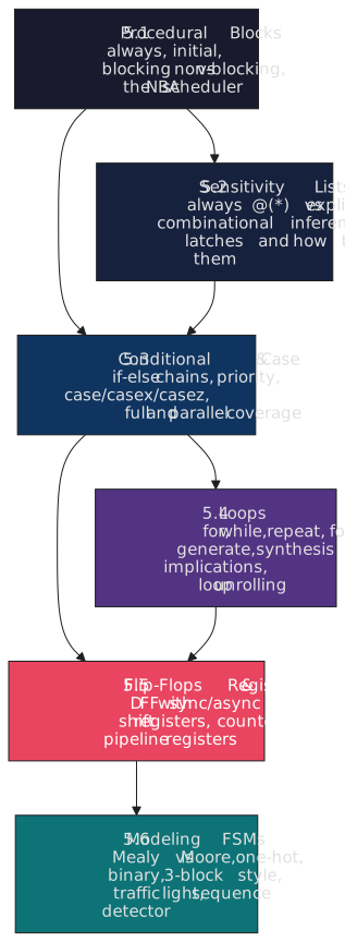
| Section | Topic |
|---|---|
| 5.1 | Procedural blocks: concurrency, always and initial, blocking and non-blocking assignment, the scheduler |
| 5.2 | Sensitivity lists: edge and level, always @(*), incomplete lists, latches |
| 5.3 | if and case: priority and parallel logic, casez, full and parallel case |
| 5.4 | Loops: for and synthesis, the other loops, patterns, generate against procedural loops |
| 5.5 | Flip-flops and registers: inference, resets, enables and loads, patterns, pipelines |
| 5.6 | State machines: anatomy, one, two and three-process styles, encoding, three worked examples |
Section 5.1 is the engine room. Sections 5.2 and 5.3 apply procedural code to combinational logic and to the latch you did not mean to build. Section 5.4 is loops. Section 5.5 is the sequential building blocks, and 5.6 is state machines, which is where all of it comes together.
What you will build
| Design | Section |
|---|---|
parity generator with a for loop |
5.4 |
| D flip-flop with synchronous and with asynchronous reset | 5.5 |
| parameterised shift register | 5.5 |
| up/down counter with enable, load and clear | 5.5 |
| a pipeline with valid signals | 5.5 |
| traffic-light controller in three styles | 5.6 |
| serial sequence detector, Mealy, overlapping | 5.6 |
| vending machine with datapath and control | 5.6 |
Every design comes with a testbench that dumps a waveform file, so you can watch the registers in GTKWave.
Tools
Same as Module 4: Icarus Verilog and GTKWave.
iverilog -o sim tb_design_name.v design_name.v
vvp sim
gtkwave tb.vcd
Every testbench in the module has
$dumpfile("tb.vcd");
$dumpvars(0, tb_design_name);
in its initial block; the 0 means every level of the hierarchy. Commercial simulators use their own compressed waveform formats because VCD files get large, but the idea is the same.
Section 5.1 opens with a module containing two always @(*) blocks that read each other’s outputs, and asks what it does. The answer is not what a programmer expects, and seeing why is the first step. Start at 5.1.