for Loops and Synthesis
Section 5.3 ended with a for loop inside a priority encoder. This section is about loops properly, and it starts with the one idea that makes them make sense in hardware: a for in RTL does not run. It is unrolled, once, when the design is elaborated, and what is left is $N$ copies of its body, side by side, all working at once.
The software picture, and why it fails
A C programmer reads
int parity = 0;
for (int i = 0; i < 8; i++) {
    parity ^= data[i];
}
as eight passes through time, one after another. The Verilog equivalent produces eight XOR gates, wired in a chain, all present and all computing continuously. There is no first pass. There is a circuit.
What a synthesisable loop needs
The synthesiser has to unroll the loop completely before it can build anything, so the bounds must be constants: literals, parameters or localparams, never a signal. The index is an integer. The body must itself be synthesisable, and the loop must terminate. A loop whose bound is an input port cannot be unrolled, because the tool would not know how many copies to make, and it is rejected with a message about a non-constant bound.
A parity generator
The parity of a word is the XOR of its bits:
$$P = b_{N-1} \oplus b_{N-2} \oplus \cdots \oplus b_0$$
`timescale 1ns / 1ps
`default_nettype none

module parity_gen #(
    parameter N = 8
) (
    input  wire [N-1:0] data_in,
    output reg          parity_out    // 1 when the number of ones is odd
);

    integer i;

    always @(*) begin
        parity_out = 1'b0;
        for (i = 0; i < N; i = i + 1) begin
            parity_out = parity_out ^ data_in[i];
        end
    end

endmodule
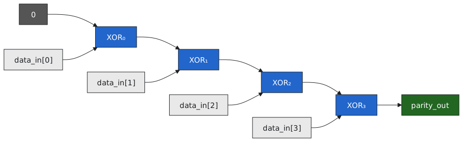
The accumulator starts at 0 and each iteration XORs one more bit in. For $N = 4$ the tool sees
parity_out = 0 ^ data_in[0]
parity_out = parity_out ^ data_in[1]
parity_out = parity_out ^ data_in[2]
parity_out = parity_out ^ data_in[3]
which is a chain of XOR gates (Figure 1), and it will usually rebalance the chain into a tree of depth $\log_2 N$, because the function is the same and the tree is faster.
This is the ^data_in reduction of section 4.3 written out, and the reduction is what you would write in practice. The loop form is here because it shows what unrolling means.
Counting ones
`timescale 1ns / 1ps
`default_nettype none

module popcount #(
    parameter N = 8
) (
    input  wire [N-1:0]           data_in,
    output reg  [$clog2(N+1)-1:0] count_out    // 0 to N needs clog2(N+1) bits
);

    integer i;

    always @(*) begin
        count_out = {$clog2(N+1){1'b0}};
        for (i = 0; i < N; i = i + 1) begin
            count_out = count_out + {{($clog2(N+1)-1){1'b0}}, data_in[i]};
        end
    end

endmodule
The loop reads as $N$ additions in sequence. The tool does not build $N$ adders in a line; it unrolls, sees one combinational expression, and builds an adder tree, the same carry-save structure as the Wallace tree of section 2.3. You write the simple accumulation; the tool does the arithmetic.
Parameters
The point of the loop is that the width is a parameter:
parity_gen #(.N(8))  u_p8  (.data_in(data8),  .parity_out(p8));
parity_gen #(.N(32)) u_p32 (.data_in(data32), .parity_out(p32));
One module, no edits, and the loop unrolls to 8 or 32 gates as needed. Once the loop-as-replicator picture is in place you write width-independent modules by habit, test them at a convenient size and instantiate them at whatever size the system wants. Hand-written repetition, thirty-two nearly identical lines, is what a reviewer flags.
A testbench
`timescale 1ns / 1ps
`default_nettype none

module tb_parity_gen;

    localparam N = 8;

    reg  [N-1:0] data_in;
    wire         parity_out;

    parity_gen #(.N(N)) u_dut (.data_in(data_in), .parity_out(parity_out));

    initial begin
        $dumpfile("tb_parity_gen.vcd");
        $dumpvars(0, tb_parity_gen);
    end

    function automatic compute_parity;      // the reference, in simulation
        input [N-1:0] d;
        integer k;
        begin
            compute_parity = 1'b0;
            for (k = 0; k < N; k = k + 1)
                compute_parity = compute_parity ^ d[k];
        end
    endfunction

    integer fail_count, test_num;

    initial begin
        fail_count = 0;
        for (test_num = 0; test_num < (1 << N); test_num = test_num + 1) begin   // all 256
            data_in = test_num[N-1:0];
            #10;
            if (parity_out !== compute_parity(data_in)) begin
                $display("FAIL: data_in=%b expected %b got %b", data_in, compute_parity(data_in), parity_out);
                fail_count = fail_count + 1;
            end
        end
        if (fail_count == 0)
            $display("PASS: all %0d vectors.", 1 << N);
        else
            $display("FAIL: %0d failures.", fail_count);
        $finish;
    end

endmodule
The testbench has loops too, in the function and in the stimulus, and they do run sequentially, because simulation is a program. The constant-bound rule is a synthesis rule; in a testbench a loop can do what it likes.
When you write a synthesisable loop you are describing a structure, a repeated pattern of gates and wires, not a computation that happens. Seen that way the constant-bound rule is obvious: you need to know how many copies to build before any data arrives. The next article is about the other three loops, and why they live in testbenches.