How TritonCTS Builds a Tree

Section 5.3 names the tool the whole module has been building towards: TritonCTS, the clock tree synthesis engine inside OpenROAD, and the one OpenLane invokes when the flow reaches the CTS stage.

It is also time to switch reference designs. Modules 2 to 4 used alu8, which has a thin register layer around a combinational core. That was fine for synthesis, floorplanning and placement, but it has no clock tree story worth telling. From here through Module 6’s routing and Module 7’s timing closure the reference design is the UART controller from the Verilog course’s Module 10 capstone, uart_top: a transmit baud generator, a receive baud generator running at 16x oversampling, and separate transmitter and receiver FSMs. It has real sequential depth, dozens of flops across several distinct blocks, which is exactly the kind of design where clock tree quality matters.

Cluster, then buffer

TritonCTS builds the tree bottom-up in two conceptual phases rather than starting at the source and working outwards.

Phase one is clustering. TritonCTS takes every clock sink, every flop’s clock pin, and its location from the completed placement, and groups nearby sinks into clusters. A cluster’s sinks will share one local buffer, so keeping physically close sinks together keeps that buffer’s fanout wiring short and its latency spread small.

Phase two is bottom-up buffered tree construction. Starting from those clusters, TritonCTS inserts a buffer to drive each one, then groups those buffers into higher-level clusters, inserts another layer of buffers to drive them, and repeats until it reaches a single root buffer near the clock’s entry point. The result looks structurally like the balanced trees from Section 5.2, but built by an algorithm reacting to this design’s actual sink locations rather than drawn as an idealised shape.

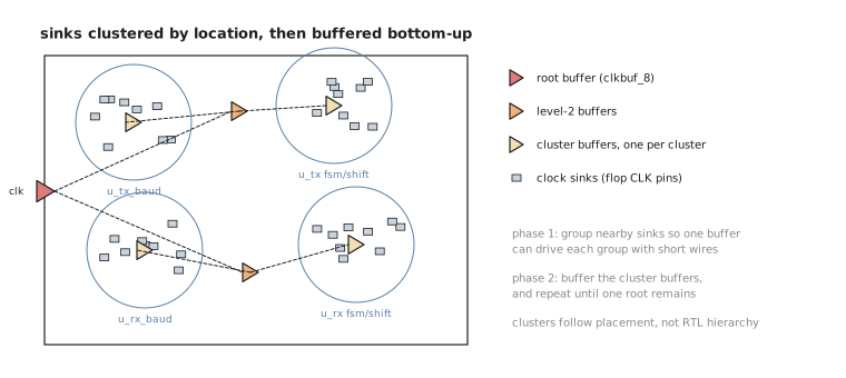
Sinks clustered by location, then buffered bottom-up — Figure 1: The UART's flop clock pins grouped into four clusters by placement, each with its own buffer; two level-2 buffers drive pairs of clusters, and one root buffer drives those.

For the UART this maps naturally onto its own hierarchy. The transmit baud counter’s bits are placed close together, the receiver FSM’s shift register and bit counter form another natural cluster, and so on. TritonCTS does not know or care that these groups correspond to RTL module boundaries. It reacts purely to physical proximity. That said, well-organised RTL with compact, coherent sub-blocks often does place into coherent clusters, which is one more reason clean hierarchical RTL pays off all the way through the physical flow.

The config knobs

OpenLane exposes TritonCTS through a handful of config.json fields. The ones you will actually touch in this module:

{
  "CTS_TARGET_SKEW": 150,
  "CTS_TOLERANCE": 100,
  "CTS_SINK_CLUSTERING_SIZE": 25,
  "CTS_SINK_CLUSTERING_MAX_DIAMETER": 50,
  "CTS_ROOT_BUFFER": "sky130_fd_sc_hd__clkbuf_16",
  "CTS_CLK_BUFFER_LIST": [
    "sky130_fd_sc_hd__clkbuf_2",
    "sky130_fd_sc_hd__clkbuf_4",
    "sky130_fd_sc_hd__clkbuf_8"
  ]
}

Read these the way you read any OpenLane config field, as targets and constraints handed to the tool, not as instructions for where to put a buffer:

CTS_TARGET_SKEW is the worst-case skew, in picoseconds, TritonCTS tries to achieve. A target, not a guarantee. The achieved value in the summary report may land close to it but not on it.
CTS_TOLERANCE is how much deviation from the target TritonCTS accepts before it keeps iterating on the tree.
CTS_SINK_CLUSTERING_SIZE and CTS_SINK_CLUSTERING_MAX_DIAMETER control phase one directly: how many sinks a cluster may hold, and how spread out, in microns, a cluster may be before TritonCTS splits it.
CTS_ROOT_BUFFER and CTS_CLK_BUFFER_LIST name the cell used at the root and the buffer variants, with their different drive strengths, TritonCTS may pick from at each level. This is the buffer sizing tradeoff from the previous article made concrete.

Notice that CTS_TARGET_SKEW is written before the tool has seen the placement. TritonCTS does not know in advance whether 150 ps is easy or nearly impossible for this floorplan and sink distribution. It finds out by building the tree, which is why the run two articles from now produces an achieved skew you compare against the target, not a number you could predict from the config.

Practice Exercise

Open designs/uart_top/config.json, or imagine it if you do not have a checkout handy, and find the CTS keys above. What happens, conceptually, if you set CTS_SINK_CLUSTERING_MAX_DIAMETER to an unrealistically small value like 2 um on a design whose flops are spread across a floorplan several hundred microns wide?

Solution

TritonCTS is forced into a very large number of very small clusters. Almost no two sinks fall within a 2 um diameter on a floorplan hundreds of microns across, so nearly every sink ends up in its own cluster. That means far more cluster-level buffers than needed, extra tree levels, extra area and power spent purely on clock buffering, and probably a harder time hitting CTS_TARGET_SKEW, since the tree is now shaped by an artificial constraint rather than the design’s real layout. The knob should reflect real sink density for the specific design.

You now know the mechanics TritonCTS uses and the knobs that steer it. Before running it, the next article covers a technique that looks like it fights everything Section 5.1 taught: useful skew, deliberately unbalancing the tree to help specific paths.