How Skew Eats Setup Margin

Recall the setup check from the Verilog course’s STA lesson. A launching flop’s data travels through combinational logic, arrives at the capturing flop, and has to be stable for the setup time before the next clock edge, all within one period. That check quietly assumed both flops see the edge at the same time. Now that you know skew is real, it is time to remove that assumption and see what changes.

The setup equation with skew made explicit

The ideal-clock setup check was

$$T_{clk} \geq t_{comb} + t_{setup}$$

Once the launching and capturing flops can have different latencies, the capturing edge does not necessarily arrive exactly one period after the launching edge. It can be a little earlier or later, by the skew between the two. In the worst case for setup, the capturing register’s clock arrives earlier than the launching register’s, shrinking the window, and skew subtracts directly from the margin:

$$\text{Slack} = T_{clk} - (t_{comb} + t_{setup} + \text{skew})$$

Read it the way a timing engineer does. (T_{clk}) is the whole budget for one period. (t_{comb}) and (t_{setup}) are unavoidable costs the logic and the library cells impose. Skew is now a third cost sitting alongside them and competing for the same budget. Every picosecond of skew is a picosecond the combinational logic no longer has room to spend.

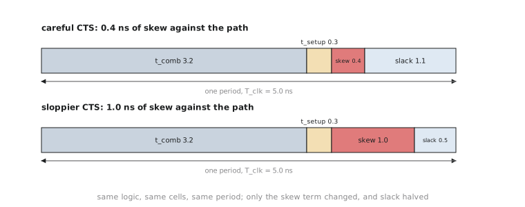
This is why “we added more logic between two registers” and “the clock tree got worse” are, from pure timing arithmetic, the same kind of problem. Both eat the same budget in the same equation. A physical designer who thinks only about logic delay and ignores the clock tree is reading half the equation.

Worked example

A design has a 5 ns period. One register-to-register path has 3.2 ns of combinational delay, the capturing flop needs 0.3 ns of setup time, and the post-CTS report shows 0.4 ns of skew working against this path.

$$\text{Slack} = 5.0 - (3.2 + 0.3 + 0.4) = 5.0 - 3.9 = 1.1,\text{ns}$$

Positive slack, so the path passes with 1.1 ns to spare. Now watch what happens if a less careful CTS run produces 1.0 ns of skew on the same path:

$$\text{Slack} = 5.0 - (3.2 + 0.3 + 1.0) = 5.0 - 4.5 = 0.5,\text{ns}$$

Same logic, same cell, same period. The only thing that changed is skew, and slack dropped by more than half. Nothing about the RTL is different. This is purely a physical design outcome, which is why CTS quality is a first-class timing lever and not a formality you run on autopilot between placement and routing.

It is also why useful skew, in Section 5.3, is a real technique and not a contradiction in terms. If skew only hurts a path when it works against the capturing register, it can just as easily help a path when it works in the capturing register’s favour. Skew is signed and path-specific. The same value can be harmless, or helpful, on a different path in the other direction, and any slack calculation that treats it as a flat universal penalty will mislead you.

Practice Exercise

A path has a 4.0 ns period, 2.6 ns of combinational delay, a 0.25 ns setup requirement, and 0.35 ns of skew working against it. Compute the setup slack. Does the path pass?

You now have the complete quantitative connection between skew and setup slack. Section 5.2 turns to the physical structures, H-trees, meshes and buffered branches, that clock tree synthesis builds to keep this skew term as small, or as deliberately shaped, as the design needs.