Inspecting Your First GDS File
In the previous article we confirmed that uart_top.gds exists and has the right top cell. That is a fact about a file. In this article we open it and look at what eight modules of work produced.
Opening the file
klayout runs/uart_full/results/final/gds/uart_top.gds &
Three parts of the window matter straight away.
The layers panel lists every layer and datatype pair used in the file, read from the stream itself. With no layer properties loaded, KLayout shows them as bare numbers like 68/20 in its own default colours, which is the point from the first article made visible: colour is a viewer setting, not part of the GDS.
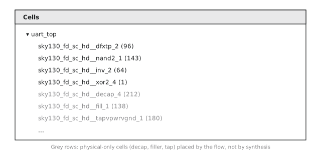
The cell list shows uart_top at the top, with every cell it uses underneath and how many times, as in Figure 1.
The layout view itself, at full zoom-out, looks like dense texture: every layer on top of every other, with no way to tell one polygon’s purpose from another’s.
Zooming in
Zoom in to a few neighbouring standard cells and the texture turns into something recognisable: diffusion rectangles, thin poly strips crossing them, small contact squares, li1 and met1 shapes connecting everything. This is as close as a digital designer gets to seeing the chip. Every polygon here becomes a feature on a photomask in Section 9.4.
Try KLayout’s ruler (press k, or pick the ruler tool, and click two points). Measure the height of a standard cell row, 2.72 µm for the HD library, or the pitch of the met1 tracks. It is your first measurement taken directly from your own finished layout rather than read from a report, and it connects back to the floorplan decisions of Module 3.
The netlist tells you what connects to what. The GDS tells you where, down to the polygon. Neither file answers both questions on its own, which is why the next section looks at tools that link the two.
When everything looks grey or oddly coloured in a fresh GDS, beginners often think the streamout went wrong. Nearly always, it is simply that no SKY130 layer properties file (.lyp) has been loaded. That is a viewer setting, fixed in the next article, not a problem with the GDS.
Practice Exercise
In the cell list of Figure 1, the counts for decap_4, fill_1 and tapvpwrvgnd_1 are larger than those of most logic cells. Where do these cells come from, and do they make up a large share of the GDS’s polygons?
Solution
They are physical-only cells added by the flow, not by synthesis. The tap cells (tapvpwrvgnd_1) were placed during floorplanning in Module 3 to tie the wells and substrate to the supplies at regular intervals. The decap and filler cells were placed by the fill insertion step in Module 8.5 to fill the empty row sites. They are numerous because they appear in every row, often many times.
They are not a large share of the polygons, though. Each is a small, simple cell, mostly well, implant and rail shapes, and like every cell its geometry is stored once and referenced many times. They are also not the metal fill for CMP density from Module 8.5, which is loose dummy metal on the routing layers. So “how many instances are in my GDS” and “how much of the geometry is logic” are different questions, and neither tells you how big the file is.
In the next article we load a proper SKY130 layer palette in KLayout and learn to read the layer stack one layer at a time.