What a GDS File Actually Is

In the last module uart_top passed every physical check: DRC, LVS, antenna, IR drop and density. In this module we deal with the file that carries it to the fab. That file is GDSII, and in this article we look at what is inside it.

The first thing to get straight is that a GDS file is not a picture of your chip. It has no colours and nothing you would recognise in an image viewer. It is a binary stream of records describing exact geometry on numbered layers, arranged in a hierarchy. It is a database, not a drawing.

A stream of records

GDSII (Graphic Design System II) dates back to Calma in the 1970s. A newer format, OASIS, exists and is used for very large designs, but GDSII is still the everyday handoff format, and it is what open flows like this one produce. The file is a sequence of typed, length-prefixed binary records. A viewer or a mask data tool reads them in order and rebuilds the design.

These are the records you will actually reason about:

Notice what is missing. There is no netlist and no “this is an inverter”. Apart from optional text labels on pins, GDSII knows only layers, polygons and structure references. Everything about why the polygons exist lives in other files: the netlist, the LEF and DEF. GDSII is the geometric truth a fab needs and nothing more.

Hierarchy

A design with 12,000 cell instances built from 50 different cell types does not need 12,000 copies of every polygon. It needs 50 structure definitions, each holding its cell’s geometry once, and 12,000 small SREF records, each just a name, a position and an orientation. This is why GDS files for designs with millions of instances stay a manageable size.

Take a tiny example: a cell INV_X1 placed twice inside a parent cell BUF_PAIR. Written out as readable text (the real file is binary, but every GDS tool rebuilds this structure from it), it looks like this:

BGNSTR  INV_X1
  BOUNDARY  layer=diff   XY=(...)
  BOUNDARY  layer=poly   XY=(...)
  BOUNDARY  layer=met1   XY=(...)
ENDSTR

BGNSTR  BUF_PAIR
  SREF  SNAME=INV_X1  XY=(0,0)
  SREF  SNAME=INV_X1  XY=(5000,0)
ENDSTR

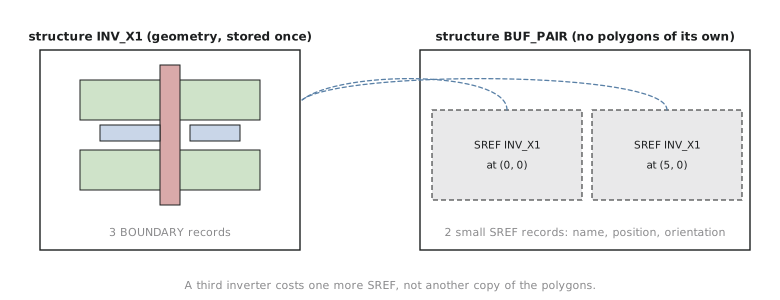
INV_X1’s polygons are written once. BUF_PAIR has no polygons of its own, only two references, as Figure 1 shows. A third inverter would cost one more SREF, not another copy of three BOUNDARY records. (In a real SKY130 file the layers are numbers, for example 68/20 for met1 drawing; the names above are for readability.)

Mask data preparation houses generally prefer hierarchical data for large designs, because a flattened file, with every instance expanded into raw polygons, can become enormous and slow to process. Some downstream steps flatten internally anyway, but the file you hand over normally keeps its hierarchy.

A common beginner’s mistake is to open a GDS and expect it to look like something. Colours, fill patterns and layer names are properties of the viewer, set by a separate layer properties file. The GDS itself only stores a layer number and a datatype number for each shape. The human-readable names and colours are added from outside, every time.

Practice Exercise

A design uses 50 different cells and has 12,000 placed instances. Why does its GDS file size depend mainly on those two numbers, rather than on the total polygon count you would get if every instance were flattened?

In the next article we write the GDS for the verified uart_top layout with Magic, and confirm it contains what we expect.