Why Post-Route Timing Differs From Every Earlier Estimate
In the previous article we saw one UART path lose most of its margin once the real route was known. If you have been following closely you may be a little annoyed by now. Module 2 gave you a synthesis timing report, Module 4 a post-placement report and Module 5 a post-CTS report, and each one was presented as “the timing report”. Now all of them are being demoted to “not the real number”. In this article I want to explain what those earlier reports were actually worth.
They were worth a lot. Each one ruled out whole classes of problems before you spent hours on a stage that would only make them harder to fix. But each one answered a narrower question than “will the finished chip meet timing”, and knowing exactly which question each stage answered is the quickest way to learn how much to trust any timing number a tool gives you.
What each stage actually knew
Synthesis (Module 2). Yosys and the synthesis STA run had no physical information at all: no floorplan, no placement, not even a die size. Wire load came from a wireload model, a statistical table that says “a net with N fanout pins in a design of this size typically has about this much capacitance”. It is a reasonable first guess and nothing more. Two nets with the same fanout can end up with very different lengths depending on where placement puts their endpoints.
Placement (Module 4). Once cells had real coordinates, the estimate improved a lot. Wire length could be approximated from the distance between a driver and its loads, usually as a half-perimeter wirelength, and turned into an RC estimate. That is much better than a wireload table, but it is still not a route. It assumes something close to a direct connection and knows nothing about the detour a real router will take around a blockage or a congested channel.
Post-CTS (Module 5). The clock got much more accurate here. TritonCTS inserts the real clock buffers and fixes the tree’s topology and buffer positions, so clock latency and skew from this stage are close to final even though the clock wires themselves are still estimated from that topology. Ordinary signal nets, including parity_net, were still running on the placement estimate. CTS reduces the uncertainty in the clock, not in the data path.
Post-route (this module). Every net, clock and signal, now has an actual route: real layer assignments, real widths and real neighbours to couple to. This is the first point in the flow where a net’s load and delay are computed from the design’s real geometry instead of from a model.
Tracking one path across the course
Here is the last stage of the parity_net path from the previous article, _2204_ driving parity_net, with the delay each stage reported (or would have reported), and the load it assumed:
| Stage | Load assumed on parity_net |
Delay of _2204_ + parity_net |
Status |
|---|---|---|---|
| Synthesis (wireload model) | ~20 fF | ~0.62 ns | Estimate |
| Post-placement (distance estimate) | ~35 fF | ~0.84 ns | Estimate |
| Post-CTS (signal nets still estimated) | ~45 fF | 1.02 ns | Estimate |
| Post-route (extracted) | 118.6 fF | 1.95 ns | Measured |
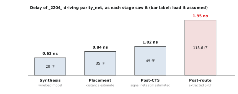
Figure 1 shows the trend. Each estimate moved closer to the final value, but none reached it, and they all erred in the same direction, because the real route was longer than any earlier stage assumed. The delay tracks the load almost exactly, which is the point from the previous article: a longer route mostly costs capacitance on the driver. This pattern is not a law (the practice exercise in the previous article had a net that came out better than estimated), but it is common enough that experienced engineers treat pre-route slack as optimistic until proven otherwise.
This is why every real physical design flow insists on a full signoff STA pass after routing, however clean the post-CTS numbers looked. A design that met timing at every earlier checkpoint can still fail after routing. The earlier reports did not lie to you. They were answering a narrower question.
The mistake to avoid is treating an early report as permission to stop thinking about timing. A clean synthesis report tells you the logic is not pathologically deep. It tells you very little about whether the routed design will meet its clock.
Practice Exercise
A different UART net reports these stage delays (driver plus wire) across the flow: synthesis 0.20 ns, post-placement 0.48 ns, post-CTS 0.51 ns, post-route 0.33 ns. Build the same tracking table for this net and explain in one or two sentences what this pattern shows that the parity_net pattern did not.
Solution
| Stage | Delay | Status |
|---|---|---|
| Synthesis | 0.20 ns | Estimate |
| Post-placement | 0.48 ns | Estimate |
| Post-CTS | 0.51 ns | Estimate |
| Post-route | 0.33 ns | Measured |
Here the estimates climbed through placement and CTS, then dropped once the real route was known. The router found a more direct path than the placement estimate assumed. This is the opposite of parity_net, and it supports the point from the previous exercise: pre-route estimates are not reliably pessimistic or reliably optimistic, they are uncertain in both directions until a real route exists. The only way to know which way a net moves is to route it and extract it.
With the reason for post-route differences settled, the next article covers a second distinction that matters just as much at signoff: graph-based and path-based timing analysis, and when a design needs the slower, more exact one.