Setup and Hold, Now With Real Wire Delay
In the previous module we finished routing the UART. Every net now has real metal at exact coordinates, with exact widths, exact spacing to its neighbours and an exact length. In this article we will see what that does to the timing numbers we have been trusting since synthesis.
Every slack figure this course has shown you so far carried a footnote that no tool prints: “assuming the wires behave the way we predicted”. Synthesis guessed wire load from a statistical wireload model. Placement refined the guess from the distance between placed cells. Post-CTS timing knew the clock tree well, but signal nets were still estimated. At every stage one part of the timing equation was a model output, not a measurement. After routing it can finally be measured.
The inequalities have not changed
Recall the setup and hold checks from the Verilog course. For a path launching at flop A and capturing at flop B:
$$T_{clk} \geq t_{clk\text{-}to\text{-}Q} + T_{comb} + t_{setup}$$
$$t_{clk\text{-}to\text{-}Q} + T_{comb} \geq t_{hold}$$
None of this is different after routing. What is different is what sits inside $T_{comb}$. That term has always been cell delay plus wire delay, and the cell delay itself depends on how much capacitance each cell has to drive. Until now both the wire and that capacitance came from a model. Now they come from the routed layout.
One point is worth getting right early, because it confuses a lot of people. In a process like SKY130, at the lengths a small block like the UART uses, the resistance of a wire is small and its own RC delay is a few picoseconds. What a longer route really costs is capacitance: every micron of metal adds load that the driving cell has to charge. So when the route turns out longer than predicted, most of the extra delay shows up in the driving cell’s delay, not in the wire line of the report. We will see this directly in the SPEF in Section 7.2.
One path, two numbers
Here is the path this whole module follows. It starts at the last bit of the UART’s receive shift register, goes through a small XOR tree that computes parity, and ends at the parity-error flop. The last XOR, instance _2204_, drives a net called parity_net into that flop.
Before routing, the tool estimated the delay of this last stage (_2204_ charging parity_net, plus the wire itself) at 1.02 ns, based on a load of about 45 fF. After routing, parity_net turned out to be a long route. It has to cross from the datapath area to the control logic and dodge other nets on the way, and the extracted load is 118.6 fF. With that load the same stage takes 1.95 ns.
The numbers in this module’s worked path are representative of what OpenSTA reports for a design like this, not a copy of one particular run. They are chosen so the arithmetic is easy to follow and so the path does something interesting later on.
Notice the direction of the error. Pre-route estimates are more often optimistic than pessimistic, because they assume a fairly direct route and know nothing about the detours real routing needs for congestion and design rules. This is why “it met timing at placement” is not the same statement as “it meets timing”.
Recomputing slack with the real number
The clock period, set back in Module 2’s SDC, is a deliberately tight 4.0 ns (250 MHz), so that this module has real closure work to do. The rest of the path, the clock-to-Q of the launching flop and the three XOR stages before _2204_, contributes a fixed 1.57 ns. On the required side, clock uncertainty (0.15 ns) and the capturing flop’s setup time (0.14 ns) come off the 4.0 ns period, which leaves a required time of 3.71 ns.
| Last stage used | Total arrival | Required time | Slack | |
|---|---|---|---|---|
| Pre-route estimate | 1.02 ns | 1.57 + 1.02 = 2.59 ns | 3.71 ns | +1.12 ns |
| Post-route, extracted | 1.95 ns | 1.57 + 1.95 = 3.52 ns | 3.71 ns | +0.19 ns |
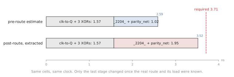
The path still meets timing, but the margin dropped from a comfortable 1.12 ns to 0.19 ns, as Figure 1 shows. Nothing about the logic changed and nothing about the clock changed. An estimate was replaced by a measurement, and the measurement was worse.
Do not read “still positive” as “done”. A path at +0.19 ns on a 4.0 ns clock has almost no room left for what this module still has to check: other process corners, temperature and supply voltage. We will meet this path again in Section 7.3, and it will not stay positive everywhere.
Practice Exercise
A different UART path runs from the baud-rate tick generator to the enable input of the transmit state machine. Its last stage (driver plus wire) was estimated at 0.42 ns before routing, and comes back at 0.39 ns after extraction. The rest of the path contributes a fixed 3.15 ns, and the required time is 3.71 ns. Does the margin get better or worse after routing, and what does that tell you about pre-route estimates?
Solution
Pre-route arrival is 3.15 + 0.42 = 3.57 ns, so slack is 3.71 − 3.57 = +0.14 ns. Post-route arrival is 3.15 + 0.39 = 3.54 ns, so slack is 3.71 − 3.54 = +0.17 ns.
The margin improved slightly. The real route for this net was shorter, or picked up less load, than the estimate assumed. So pre-route estimates are not always optimistic. They are simply unreliable, sometimes worse than reality and sometimes better, and you cannot tell which without extracting the real geometry. That uncertainty, more than any bias in one direction, is why signoff timing has to use extracted parasitics.
Before we get into extraction itself, the next article walks stage by stage through what each earlier timing report in this course did and did not know, and why routing is the last stage that can surprise you.