Inspecting Special Nets in KLayout

Two articles of reasoning about why power and clock nets are routed differently. Reasoning is good, but nothing beats looking at the geometry. This one is a lab: open the UART’s routed layout in KLayout, the independent viewer this course uses precisely because it is not the tool that did the routing, so what you see is a second opinion, and pick the special nets out of the crowd.

Getting the routed design into KLayout

After run_routing completes, OpenLane writes a routed DEF, and later a streamed GDS once you reach Module 9. KLayout opens either. For this lab, open the routed DEF with the SKY130 layer properties file so each layer renders in a distinct, labelled colour:

klayout -l sky130A.lyp \
    designs/uart/runs/routing_run_01/results/routing/uart.def

Without the -l flag you would be staring at undifferentiated grey rectangles with no way to tell met2 from met4 at a glance. KLayout needs the technology LEF to interpret a DEF; point it at the SKY130 tech LEF when prompted, or load the DEF through a technology that already references it.

Isolating the power grid

In the Layers panel, turn off every routing layer except the ones the grid uses, met4 and met5 per the DEF excerpt from two articles ago. What remains should match the structural description immediately: a ring tracing the full core perimeter on met5, and a series of evenly spaced straps crossing the interior on met4. Compare that with isolating an ordinary signal layer like met2: a dense, irregular tangle of short segments in different orientations with no repeating pattern, because signal nets are routed to individually optimal paths, not regular structures.

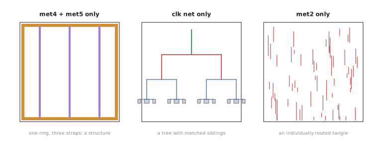
Three views of the same routed UART — Figure 1: Left, only met4 and met5 visible: one ring and three straps. Middle, only the clk net: a tree with matched siblings. Right, only met2: an individually routed tangle.

That contrast, regular perimeter-and-grid geometry on the power layers against irregular, individually shaped geometry everywhere else, is the visual signature of “built as a deliberate structure” against “routed net by net”.

Isolating the clock net

KLayout’s net highlighting, select a net by name or use the net tracer depending on version, isolates the clk net’s geometry across whatever layers it uses. You should see something distinct from a signal net’s routing too: a recognisable branching tree, a trunk splitting into roughly symmetric sub-branches, splitting again, and ending at flop clock pins, rather than point-to-point paths. It is the physical realisation of the CTS topology from Module 5 and of the DEF excerpt from the previous article. Trace two sibling branches from one fork by eye. Their lengths should look close, not arbitrary.

This visual check, isolate the power layers, isolate the clock, confirm both look structurally different from signals, is a habit working physical designers use as a quick sanity pass after a routing run, well before any formal IR drop or post-routing timing. If the grid looks thin or broken in a region, or the tree looks lopsided, that is worth investigating before you get to the reports in Modules 7 and 8. Reports give you counts and lengths. A visual pass catches structural oddities, an asymmetric clock branch, a strap that looks thinner in one region, that are obvious the moment you see them and easy to miss in a table.

Predicting before you look

Before opening KLayout, sketch what you expect when you isolate met4 and met5 for the UART’s 300 um square core, based only on the DEF excerpt: one ring on met5, three vertical straps on met4 at three x coordinates. Then open the layout and compare.

There is no single correct mismatch to report. The value is in the comparison. A physical designer builds a mental model of what geometry should be there from the reports and config already read, then uses a visual tool to confirm or refute it. If the sketch predicted a ring plus three straps and KLayout shows a ring plus three straps in roughly the same places, the grid was built as intended. If KLayout shows a fourth strap you did not expect, or one missing, that is exactly the discrepancy this habit is designed to catch.

Practice Exercise

You isolate the clock net and, tracing from the root buffer, notice one branch is visually much longer than its sibling from the same fork, inconsistent with the “roughly symmetric” expectation. Which two modules’ tools would you use, in what order, to decide whether this asymmetry is actually a problem?

Solution

First, Module 5’s post-CTS timing report: check whether the skew between the flops fed by those two branches is within budget despite the visual difference. CTS sometimes builds asymmetric branches on purpose when the flops at the ends have different loads or intrinsic delays to equalise against, so visual asymmetry alone is not proof of a problem. Second, if the post-CTS numbers look fine but you want to confirm the physical routing did not add imbalance beyond what CTS intended, Module 7’s post-routing STA with extracted parasitics measures the tree’s as-routed delay rather than CTS’s estimate, and is what catches a routing-introduced skew problem. KLayout raised the question; the timing tools answer it.

You have seen what good, structurally correct routing looks like. Section 6.5 turns to the opposite case: reading a routing report when things go wrong, starting with how to interpret a real violation report.