The Routing Grid

Module 6 starts where Module 5 left the UART: every flop has a clock, timing looks sane, and the placement database has a location for every one of the roughly 1,300 standard cells. And yet not a single signal wire exists. Every net, the ones carrying tx_data, rx_shift, baud_tick, all of it, is still a rubber-band line in the placement viewer, a straight-line guess at where a wire will eventually go.

Turning a few thousand rubber bands into physical metal without any of them stepping on each other is a genuinely hard combinatorial problem. If you tried to solve it in one shot, picking the exact track, layer and via for every net at once, the search space would be enormous, and a bad early decision for net 12 could make net 4,000 unroutable with no way to know until you were deep into the process. So the router does not do it in one shot. It works coarse to fine: global routing first, detailed routing second. This article is about the first pass.

A rough path, fast

Global routing does not touch real tracks at all. OpenROAD’s global router, FastRoute, overlays the core with a coarse grid of rectangular tiles called GCells. Think of them as neighbourhoods rather than addresses. A GCell might span dozens of routing tracks. For each net, global routing decides which sequence of GCells the wire will pass through, and roughly how many wires on each layer will need to cross each boundary between neighbouring GCells. It does not decide the exact track or via stack, and it resolves no design rule.

That is the whole point. By working at neighbourhood granularity, global routing can consider the entire design’s routing demand at once, cheaply, and catch a structural problem, “this neighbourhood has far more nets wanting through than it has room for”, while it is still a planning exercise rather than a legal-wire crisis.

Capacity, demand, and why congestion shows up here first

Each edge between two adjacent GCells has a capacity: an estimate of how many wires can cross that boundary on the available layers, from the track pitch and how much of that space is already eaten by power straps or macro blockages. As global routing routes every net it also tallies demand, how many nets want to cross that edge. Where demand exceeds capacity you have congestion, reported as overflow on that edge. You met this in Module 4 as a diagnostic run on a placement. Here it is the real thing.

Overflow is the single most useful number global routing produces. Zero everywhere means the design is, in principle, routable. Detailed routing still has to prove it can make every wire legal, but the gross traffic-jam problem does not exist. A stubborn overflow in one region, no matter how the router shuffles net order, is an early, cheap warning that something upstream, most likely placement density in that area, needs to change before detailed routing wastes hours discovering the same thing the hard way. Section 6.5 comes back to exactly this move.

Global routing is deliberately imprecise, and that is a feature. It trades exactness for the ability to see the whole design’s demand in one pass. The corresponding trap is treating a clean global routing pass as proof the design will route. It proves there is roughly enough capacity. Detailed routing still enforces every spacing, width and via rule, and a design can sail through global routing with zero overflow and hit real DRC violations once TritonRoute draws exact geometry. Global routing is necessary, not sufficient.

Sketching two coarse routes

Take a tiny 3x3 GCell grid over a corner of the UART’s core. The middle row is busy: a wide power strap and a cluster of CTS clock buffers eat most of its spare capacity, so treat that row as low capacity. Net A needs to get from row 0, column 0 to row 2, column 2. Net B needs to get from row 0, column 1 to row 2, column 1.

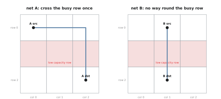
Net A must start in row 0 and end in row 2, so it has to cross the middle row no matter what. The efficient path minimises how much of that scarce row it consumes: go horizontally while still in a full-capacity row, then cross once. Row 0 column 0 to column 2, then down through row 1 column 2 to the destination, uses the busy row in one column only, against a path that zigzags through row 1 for two or three GCells.

Net B is the harder case. Source and destination are on opposite sides of the busy row, directly above and below each other. No orthogonal path avoids row 1. This is exactly the situation that produces overflow. If enough nets are in net B’s position, all needing to cross the same constrained row, that row’s capacity gets exhausted however cleverly the router orders them, and the fix is not a smarter route. It is more capacity: a different layer, less blockage, or a placement that does not crowd that row in the first place.

Practice Exercise

A GCell edge has a capacity of 12 tracks after subtracting the space used by a fixed power strap. Global routing’s first pass assigns 15 nets across that edge. Two nets are later ripped up and rerouted through a neighbouring, less loaded edge. What is the new demand on the original edge, and is it still congested?

Every one of those GCell edges has a capacity that ultimately comes from real metal layers with real track pitches. The next article walks the SKY130 metal stack layer by layer and what each one is conventionally for.