Tuning a Real Design to Convergence
This closes Module 4 by running the whole loop for real, on alu8, deliberately starting from a bad configuration so the fix is visible rather than asserted. Every report format below is one you have already read this module. The only new thing is watching them change across two runs.
Iteration 1: too aggressive
Start with PL_TARGET_DENSITY at 0.75, well above the 0.55 the previous article’s formula would suggest for alu8’s FP_CORE_UTIL = 45, chosen to produce a problem worth fixing.
% prep -design alu8 -tag placement_tune_v1
% set ::env(PL_TARGET_DENSITY) 0.75
% run_placement
Congestion report excerpt:
Layer      Resource   Demand    Usage(%)   H overflow   V overflow
li1            3840      3690      96.1%            5            2
met1           5120      5210     101.8%            3            8
met2           5120      6042     118.0%            2           14
met3           2560      2380      93.0%            0            1

[WARNING GRT-0019] Overflow found on layer met1: 11 GCell edges.
[WARNING GRT-0019] Overflow found on layer met2: 16 GCell edges.
[INFO GRT-0020] Total design overflow: 27 GCell edges (0.19% of all edges).
Pre-CTS timing, worst path:
  18.62   18.62   data arrival time
  19.85   19.85   data required time
-----------------------------------------------
  -0.42               slack (VIOLATED)
Two connected problems with one root cause. met1 and met2 are both over capacity, at 101.8% and 118.0%, against met2 alone at 105.3% in Section 4.4’s more moderate example, and the worst pre-CTS path has gone negative, a real setup violation even under the still idealised clock. Packing cells to a 0.75 target left too little local routing room in several regions, and forced legalisation into larger, less wirelength-friendly displacements in the tightest spots. That is exactly the degradation Section 4.1 warned an over-aggressive density push would cause.
Applying the loop: one knob
Following the loop exactly, one knob, PL_TARGET_DENSITY, down from 0.75 to 0.55, the value the formula actually recommended for this design.
% prep -design alu8 -tag placement_tune_v2
% set ::env(PL_TARGET_DENSITY) 0.55
% run_placement
Congestion report excerpt:
Layer      Resource   Demand    Usage(%)   H overflow   V overflow
li1            3840      3512      91.5%            0            0
met1           5120      4877      95.3%            0            0
met2           5120      4864      95.0%            0            0
met3           2560      2190      85.5%            0            0

[INFO GRT-0020] Total design overflow: 0 GCell edges (0.00% of all edges).
Pre-CTS timing, worst path:
  17.94   17.94   data arrival time
  19.85   19.85   data required time
-----------------------------------------------
   1.91               slack (MET)
Zero overflow on every layer, and the worst path swung from a 0.42 ns violation to 1.91 ns of comfortable positive slack.
The full before and after
| Metric | v1 (density 0.75) | v2 (density 0.55) |
|---|---|---|
met1 usage |
101.8% (overflow) | 95.3% |
met2 usage |
118.0% (overflow) | 95.0% |
| Total overflow edges | 27 | 0 |
| Worst pre-CTS slack | -0.42 ns (VIOLATED) | +1.91 ns (MET) |
| Total HPWL | 782,150 dbu | 818,210 dbu |
| Max legalisation displacement | 612 dbu | 38.5 dbu |
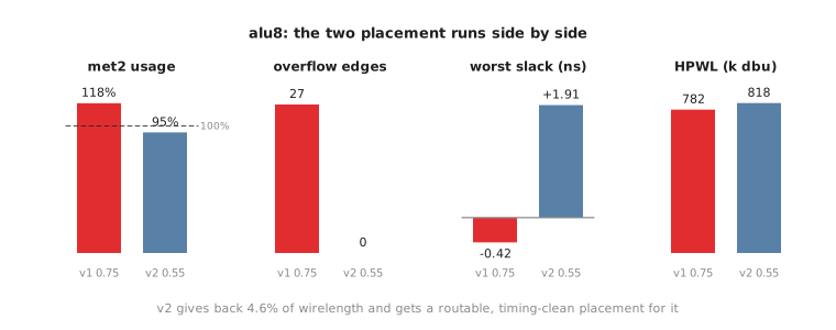
Read the last two rows carefully, because they are this module’s opening argument made concrete. v1’s aggressive packing achieved lower total wirelength, 782,150 against 818,210 dbu. Tighter packing shortens the average net, exactly as Section 4.1 predicts. But it bought that at the cost of severe congestion, a real timing violation, and legalisation forced into much larger displacements, 612 dbu against 38.5 dbu, to find legal sites in overcrowded regions. v2 gives up about 4.6% of raw wirelength in exchange for a routable, timing-clean, easily legalised placement.
This is not “v1 was wrong and v2 was right” in any absolute sense. It is the wirelength-against-congestion-against-timing conflict from Section 4.1, with a real number attached to each side for the first time in this course. Every real placement tuning decision looks like this table: a small, quantifiable cost on one axis, bought to fix a larger, more urgent problem on two others. Chasing the lowest wirelength as if it were the goal misses that. Legality, routability and timing closure are the requirements. Low wirelength is a means to a faster, smaller, lower-power chip, not an end that justifies a congested, timing-failing design with a smaller HPWL attached.
Practice Exercise
A third engineer, looking only at the two HPWL numbers in the table, argues the team should ship v1 because it has better wirelength. Write a two or three sentence response explaining why that reasoning is incomplete, using the specific numbers from this article.
Solution
Wirelength is one of three things this module has established a placement must satisfy, and v1 fails the other two outright. It has 27 GCell edges of routing overflow, meaning some nets cannot be routed as placed, a Module 6 failure waiting to happen, and a -0.42 ns pre-CTS setup violation even under an idealised zero-skew clock, one that Section 4.3’s discussion of real skew suggests would persist or worsen once a clock tree exists. A 4.6% wirelength advantage does not offset an unroutable, timing-failing design. v2 is the only one of the two usable as a foundation for Module 5.
Placement is done: legal, routable by this diagnostic’s estimate, and passing pre-CTS timing with real margin. The one deliberate gap left in every report this module has shown is the idealised, zero-delay clock. Module 5 replaces that assumption with a real clock tree, and as Section 4.3 warned, that is exactly where some of this module’s comfortably passing margins get their first real test.