The Tuning Loop
Every article in this module so far has quietly built towards one working method without naming it. Time to name it, because you will use this exact shape of workflow, not just this exact knob, at every remaining stage of the course.
The loop
- Run placement with a chosen
PL_TARGET_DENSITY. The previous article gave you a starting formula, not a final answer. - Check congestion: run the global-route estimate from Section 4.4 and scan the per-layer report for overflow.
- Check pre-CTS timing: run
report_checks(Section 4.3) and look at worst slack, remembering the ideal-clock caveat. - If both look acceptable, stop and move on to Module 5. If not, adjust exactly one knob, most often
PL_TARGET_DENSITYitself, though it could be a floorplan-level change if the problem is structural, and go back to step 1.
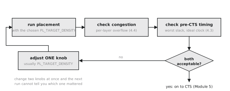
The words “exactly one” in step 4 do real work. Change two knobs at once, say PL_TARGET_DENSITY and FP_ASPECT_RATIO in the same iteration, and when the next run’s numbers improve or worsen you have no way to attribute the change to either knob. This is ordinary experimental discipline, not something specific to placement. Isolate your variable or the loop stops teaching you anything.
This is not a Module 4 thing
You will run some version of the same four steps, run, check the relevant metric, adjust one knob, rerun, at almost every remaining stage:
- Module 5 (CTS): run TritonCTS, check post-CTS skew and hold slack, adjust a clock buffer or CTS target, rerun.
- Module 6 (Routing): run detailed routing, check DRC violations and unrouted nets, adjust a routing layer or congestion knob, rerun.
- Module 7 (Timing Closure): run signoff STA, check slack across corners, apply an ECO such as a buffer insertion or a resize, rerun.
Placement is simply the first stage where the loop becomes necessary, because it is the first stage where one well-understood knob has a clear, predictable effect on two competing, checkable outcomes. Learn to run it with discipline here and the mechanics carry over. Only the tool and the metric change.
Experienced physical design engineers rarely describe their day as designing a placement. They describe it as tuning a placement or closing on a config, language that reflects exactly this loop. The OpenLane config.json accumulates small, deliberate adjustments over several iterations, each justified by a specific report finding, rather than being chosen up front and left alone. So a bad first-iteration result is not a sign the approach is broken. It is step 2 of a loop that is supposed to take a few passes, telling you where to adjust next.
Tracing a tuning log
A design goes through four iterations, tuning only PL_TARGET_DENSITY:
| Iteration | PL_TARGET_DENSITY | Worst met2 overflow | Worst pre-CTS slack |
|---|---|---|---|
| 1 | 0.75 | 18% | -0.42 ns (fails) |
| 2 | 0.65 | 11% | -0.10 ns (fails) |
| 3 | 0.58 | 3% | +0.12 ns (passes) |
| 4 | 0.55 | 0% | +0.38 ns (passes) |
At which iteration would you stop, and would you have been justified stopping one earlier?
Iteration 4 is the clean stopping point: zero overflow and comfortably positive slack. Iteration 3 technically passes both checks, 3% overflow is small and slack is barely positive, and a time-pressed engineer might reasonably stop there. But iteration 4 buys noticeably more margin on both metrics for a small further reduction in density, which is normally worth one more placement run. There is no universally correct answer. It is a judgement about how much margin is enough, and the loop’s job is to inform that judgement with real data rather than guesswork.
Practice Exercise
A fifth iteration at PL_TARGET_DENSITY = 0.50 reports 0% overflow and +0.41 ns slack, both very slightly better than iteration 4. Is it worth continuing past this point? What would you want to know before deciding?
Solution
Probably not, on these numbers alone. The improvement from 0.38 ns to 0.41 ns is marginal, and both already clear the acceptable bar. Before deciding, check one thing the table does not show: total wirelength (HPWL) at each density. Lowering PL_TARGET_DENSITY further spreads cells out more, which starts increasing wirelength for diminishing congestion and timing benefit, exactly the tradeoff the module’s closing article works through with real numbers. Diminishing returns on the metrics you are optimising, combined with a real cost on one you are not tracking, is usually the signal to stop.
You have seen the loop described and traced through a hypothetical log. The module’s final article runs it for real: start alu8 at a deliberately aggressive density, watch it fail, tune it down, and confirm the fix with the same reports you have used all module.