How Synthesis Optimizes for Timing
The previous article wrote the constraints. This one is about what the tool does once a create_clock tells it a particular path is running out of room.
Lever 1: gate sizing
Every gate in a standard cell library exists in several physical sizes. A “2x” or “4x” drive-strength inverter is not a different gate; it is the same function built with larger transistors, which switch faster at the cost of more area and more power. A tool facing a tight path will upsize the cells along that path, swapping in higher-drive versions of the same cells, trading area and power for speed on the paths that need it and nowhere else.
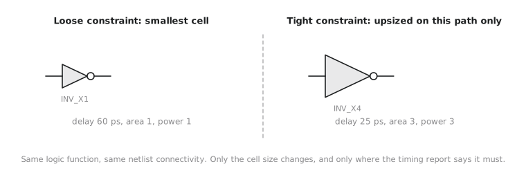
This is why two functionally identical designs synthesized against different clock targets come back with different area even though the RTL did not change. A loose constraint lets the tool use its smallest, most area-efficient cells everywhere; a tight one forces selective upsizing exactly where the critical path analysis says it is needed.
Lever 2: logic restructuring
Beyond swapping sizes, the tool can restructure the Boolean logic to reduce depth, the number of gate delays stacked in series on the critical path, even when the gate count barely changes. The classic example is a wide AND:
assign all_ready = a & b & c & d & e & f & g & h;
A literal reading builds a chain of seven 2-input ANDs in series, seven gate delays deep. A tool that knows this path is timing-critical rebuilds the same function as a balanced tree:
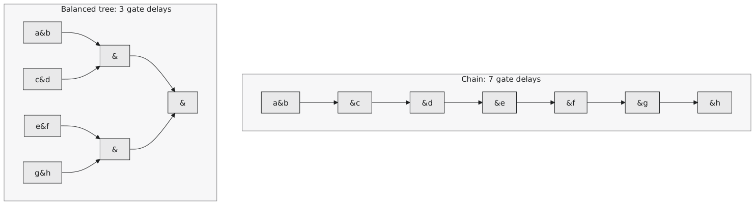
Same function, same number of 2-input gates, but the tree’s critical path is $\lceil \log_2(8) \rceil = 3$ gate delays instead of 7. This is the kind of transformation the first article in Section 8.2 called logic optimisation discovering a structure the RTL did not spell out. You wrote a chain of &; the tool, under timing pressure, rebuilt it as a tree, because they compute the same thing and a tree is shallower.
Watching a tightening constraint change the result
Put the two levers together and you get a picture of what happens as you sweep the create_clock period tighter against unchanged RTL:
| Constraint | Typical synthesis behaviour |
|---|---|
| Very loose (e.g. 20 ns for a design that fits in 5 ns) | Smallest cells, maximum resource sharing, chain-structured logic wherever it is simplest: area-optimised, since there is no timing pressure |
| Moderate (e.g. 6 ns) | Some selective upsizing and restructuring on the slower paths; most of the design stays area-optimised |
| Tight (e.g. 4.5 ns, close to the real limit) | Aggressive upsizing and tree restructuring on the critical path; resource sharing may be suppressed on the tightest paths per Section 8.2 |
| Infeasible (e.g. 2 ns, below what the logic can achieve) | Violations reported: no sizing or restructuring makes combinational logic faster than its gate-delay floor; this needs an RTL fix (pipelining, Section 7.3), not a synthesis one |
The last row matters. Synthesis-level optimisation can close a moderate gap, but it has a hard floor set by the number of logic levels the RTL requires and the fastest available gate at the process node. Once you hit that floor, the only fix is architectural, the pipelining discipline from Section 7.3: break the path across a clock boundary rather than trying to make an already-minimal combinational path faster.
This is the mechanical link to the “trust the optimiser, constrain honestly” principle in Section 8.2: an honestly tight constraint is what triggers the tool to spend area and power on upsizing and restructuring the paths that need it. A loose or missing constraint means the tool never tries, because as far as it can tell there is no pressure to.
Practice Exercise
A design meets timing comfortably at 10 ns with a compact, low-area result. The target is tightened to 4 ns, the design still meets timing, but the reported area has grown by 40 percent. Explain what most likely happened.
Solution
The RTL almost certainly did not change; only the constraint did. At 10 ns the tool had generous slack on essentially every path, so it used small, low-power cells and simple chain-style structures wherever the RTL suggested them. Tightening to 4 ns put pressure on whichever paths were closest to the new limit, and the tool responded by upsizing cells along those paths (lever 1) and restructuring deep chains into shallower trees (lever 2). Both cost area: larger cells directly, and tree restructuring often uses more total gates than a chain even though it uses fewer levels. That is the area-for-timing trade, now visible as a percentage in a real report rather than as a concept.
Gate sizing trades area and power for speed on exactly the paths a tight constraint identifies, and logic restructuring rebuilds a deep chain into a shallower tree with the same function. Both have a floor set by the RTL’s logic depth and the process’s fastest gates; past that the fix is architectural. In the next article, the last in this section, we read an actual timing report, so you can tell which of these situations you are in.